MCA

Maximum Covariance Analysis (MCA) is a widely used discriminant analysis technique for identifying coupled patterns in climate data. It works by finding linear combinations of a predictor and predictand field that maximize their covariance through singular value decomposition (SVD). MCA is particularly useful for summarizing large climate datasets into a few dominant modes of variability, revealing spatial patterns linked by teleconnections. For example, applying MCA to tropical Pacific sea surface temperature (SST) anomalies and anomalous sea level pressure (SLP) identifies El Niño-related SST patterns and the Southern Oscillation in SLP. Spy4Cast implements MCA by organizing predictor and predictand fields into space-time matrices, ensuring they share a common time dimension while allowing for spatial differences, with their covariance matrix defined as \(C = Y \cdot Z^T\).

MCA is performed with class spy4cast.spy4cast.MCA

To perform MCA on predictor, \(Y\) and a predictand \(Z\) with Spy4Cast you need to load the datasets, slice them and preprocess them first:

from spy4cast import Dataset, Region, Month, spy4cast

y = Dataset("predictor.nc", folder="datasets").open().slice(
    Region(lat0=-20, latf=20, lon0=-10, lonf=40,
           month0=Month.JAN, monthf=Month.MAR, year0=1964, yearf=1994))
z = Dataset("predictand.nc", folder="datasets").open().slice(
    Region(lat0=-10, latf=-40, lon0=-180, lonf=-100,
           month0=Month.FEB, monthf=Month.APR, year0=1964, yearf=1994))
yp = spy4cast.Preprocess(y)
zp = spy4cast.Preprocess(z)
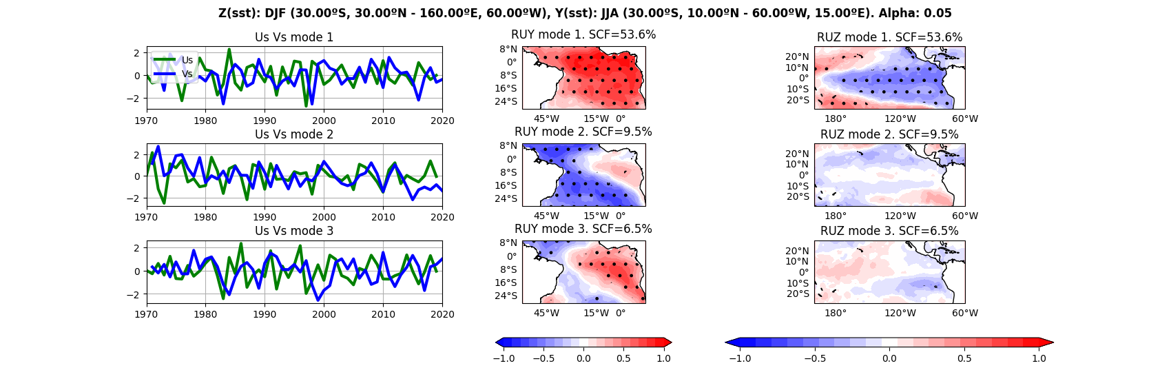
mca = spy4cast.MCA(yp, zp, nm=3, alpha=0.1)
mca.plot(show_plot=True, halt_program=True)

The following figure is an example of the figures that can be created with MCA. It is done with the code from the manual Spy4Cast Manual of example EquatorialAtlantic_Impact_Nino.ipynb